What is separable convolution, why would we use it, when can it be applied and how to get the 1D filters.
Intro
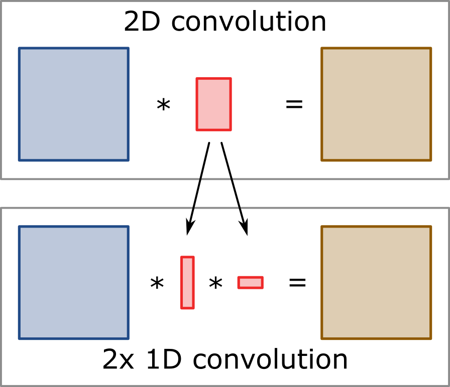
Separable convolution describes an operation where a 2D convolution procedure can be split up into two separate 1D convolutions along the two axis of the image. The 1D convolutions are thereby executed one after the other making use of the principle that convolution operations are associative. Splitting up the procedure can thereby largely reduce the amount of required multiplications and additions and therefore typically comes with a significant increase in speed. The improvement thereby depends on the size of the 2D kernel. An image with a size of M x N which is filtered with a kernel of size P x Q would thereby require a total of M * N * P * Q multiplications and additions (or combined operations) for the 2D convolution. If we move to the separable 1D approach, the complexity is reduced to M * N * (P + Q) resulting in a theoretically achievable speed up of (P * Q) / (P + Q). For a quadratic kernel (P = Q) this means that the speed up is defined as P / 2, resulting in approximately 10 fold speed up for kernels of size 21 x 21.
For computational performance and depending on your architecture it might furthermore make sense to perform two transpose operations in between the convolutions to always perform the 1D convolution along the fast axis of your array and avoid strided memory access.
The method has quite some use in convolutional neural networks where the training requires a lot of computational power, but also in image processing algorithms which require fast performance in environments such as medical imaging.
Filter separability
Not every 2D convolution can be decomposed into two separate 1D convolutions but many commonly used filters such as a Gaussian function can be split up. The property is called filter separability. To determine if your kernel can be separated, calculate the kernel as a 2D matrix and determine the rank of the matrix. If the rank is one (or close to it), you can make use of the procedure.
How to derive the individual filters?
The tool we need here is called singular value decomposition. A singular value sigma and the two singular vectors u and v can be used to described a matrix A. The most intuitive understanding is thereby that the matrix can be described as the outer product of the two vectors
\begin{equation}
A = v \otimes u
\end{equation}
So the choice is to either take your matrix and apply the singular value decomposition on your numerical matrix or try to solve the system analytically. Let’s assume that we have a filter kernel that is defined as the some of two exponential functions along the radial distance from the center:
\begin{equation}
F(r) = \beta \exp(-r^2 \cdot \sigma)
\end{equation}
Decomposing a 2D Gaussian matrix into two components is straightforward since:
\begin{equation}
\exp(-r^2 \cdot \sigma) = \exp(-(x^2 + y^2) \cdot \sigma) = \exp(-x^2 \cdot \sigma) \cdot \exp(-y^2 \cdot \sigma)
\end{equation}
This relationship shows that the equation describing the kernel can easily be decomposed into two multiplicative terms holding either x or y components. The first convolution can therefore be applied with a vector v generated from the first term and the second one along y will be applied with the second term generating the vector u.
The constant factor beta can either be applied later to the kernel or included as a multiplicative term into one of the above equations.
Read more: